Thursday 28 May 2020

Just a snapshot

I have reported previously that Nicola is working very hard on bringing AstroDMx Capture closer to a new release.
The latest features to  be added are:
  1. Allowing the software control of the video stream to be enabled for saving. This means that the gain, gamma, brightness and contrast software controls can be applied to the saved data if this function is enabled. Moreover, gain is a newly implemented software control.
  2. Allowing the capture of very high-quality Tiff, named snapshots snapshots to be captured at the click of a button into a snapshot folder within the AstroDMx_data folder.
These functions have been added to give the user more choice over what they wish to  do. There is debate as to whether gamma is required in a camera control, and has been previously pointed out, ZWO removed the gamma function from their SDK whilst QHY retained it in theirs. I think that gamma control can be useful, and so, am happy to see this software control (which works on the video feed, not on the camera) present in AstroDMx Capture.

AstroDMx Capture for Linux being used to  name the snapshots 'Moon'

The button to the right of the Snapshot button is used to name the snapshots. If several snapshots are captured, they will carry the same timestamped name with an incremented index.  For example, the 8th snapshot with the name 'Moon' will have the filename: Moon__000008__21-58-20__data.tiff .

Detail of the snapshot naming window that can be seen on top of the preview window

A single snapshot of the Moon captured by AstroDMx Capture for Linux

Closer view

This is not recommending that snapshots should routinely be used for capturing images of the Moon. The relative success will strongly depend on the seeing. This image was captured on a night when the jet-stream was far to the north of the country, so it did not have a deleterious contribution to the seeing. However, the user now has the choice.
It is far more likely that users of the software for microscopy will make use of the snapshot function.

Wednesday 27 May 2020

New features for AstroDMx Capture

New features in AstroDMx Capture 

During the current development of AstroDMx Capture for Linux, macOS and Windows, we have been in feature freeze following the implementation of motion detection, as Nicola has been substantially refactoring the code and bringing it into a single code base. However, recent experience with a nest box camera and a digital microscope has led us to make two exceptions that will facilitate the use of AstroDMx Capture for these two types of use of the software.

AstroDMx Capture for Linux streaming data from a digital microscope 
which has no camera controls

AstroDMx Capture has long had set of display controls that enable the user to change the gamma, brightness, and contrast of the display in a non-destructive way. That is, the display controls only effect the display, but not the saved data.

However, there are some cameras such as the nest box endoscope type camera that we have been using, and the digital microscope, that have minimal, or even no controls, and are in fully automatic mode. We have found that the ability to control the gamma and contrast, of the display has enabled much clearer views to be obtained of the nest box, particularly in low light.

We decided to allow the user to enable the saving of the display, software-controlled data, thus effectively adding controls to the camera. This saving function can be toggled and only applies to 8-bit data. This is effectively what capture cards do with the data streaming from an analogue video camera, providing added control over the video stream. Nicola has implemented this code and has, in addition to gamma, brightness and contrast, also implemented a software gain control.

Some camera manufacturers such a ZWO removed the gamma control from their SDK even though internally, the camera is capable of gamma control. The purists say that gamma control is not necessary because that aspect of an image can be dealt with in post processing. It is my opinion that gamma control is very useful at capture time and allows a better balance between gain and exposure control as one is able to see regions of intermediate brightness such as the region close to the terminator in a lunar image, without increasing the exposure and in the process, overexposing the brighter regions. Also, in H-alpha solar imaging, control of gamma can help see the structures that occupy various regions of the dynamic range.

Screenshot of AstroDMx Capture for Linux capturing lunar data with a ZWO ASI178MC camera, with the software controls enabled for viewing and saving, and with the gamma increased above the default for the camera


Closer view
The settings of the software video processor can be seen and they are enabled. The gamma has been set to 1.9. The default value is 1.0.

Screenshot of AstroDMx Capture for Linux capturing lunar data with a ZWO ASI178MC camera, with the software controls disabled, and with the gamma at the default for the camera
The gain and exposure were set so that there was just no saturation of the lighter parts of the image.

Closer view
The settings of the software video processor can be seen, but they are diabled

Four overlapping panes were captured as 1000-frame SER files. The best 90% of the frames in the SER files were stacked in Autostakkert!, wavelet processed in Registax 6, stitched into a single, 4-pane mosaic and post processed in the Gimp 2.10.

16.8% waxing, crescent Moon

Another feature has been added that required a slight change to the GUI. This is the addition of a Snapshot button. This will be of limited value for astronomy unless AstroDMx Capture is being used simply to stream video for outreach purposes, and an occasional snapshot is required from the session. The ability to capture individual images is of more importance for microscopy, and to some extent, visually monitored cameras.

AstroDmx Capture for Linux Streaming video from a nest box camera with no camera controls. The software controls are turned off

AstroDMx Capture for Linux streaming video from a nest box camera with no camera controls. The software controls are enabled and adjustments have been made to reveal more of the interior of the nest box.
These two shots were taken before Nicola had implemented software gain control

When the Snapshot button is clicked, a snapshot folder is created in the AstroDMx Capture Data folder and an uncompressed Tiff file is saved. The user should select ‘RAW8’ or RAW16 when connecting the camera rather than RGB, if a colour camera is being used. This will ensure that a very high-quality debayering algorithm is applied to the captured image that is superior to the one supplied in the SDK for the RGB selection. If a monochrome camera is being used, then selecting ‘MONO 8’ or ‘MONO 16’ will, of course, result in an uncompressed greyscale Tiff being saved. The time-stamped Tiff image is saved in the snapshot folder. Immediately to the right of the Snapshot button is a small button that if clicked, allows for the naming of the images to be captured by Snapshot. This name does not override the name selected for general imaging, and if the naming button is not used for snapshots, then the image name from the previous regular imaging session will be used, which may not be appropriate. It is therefore recommended that the snapshot naming button be used routinely when capturing snapshots.

Snapshot of the interior of the nestbox.

Friday 15 May 2020

Stochastic 'Lucky' Imaging of the 11.9% crescent Venus with AstroDMx Capture for Linux

A Skymax 127 Maksutov was mounted on a Celestron AVX mount. A ZWO ASI178MC camera fitted with a 2.5x Barlow was placed at the Cassegrain focus of the Maksutov.

AstroDMx Capture for Linux was running on a 9th generation, Core i7, PC Specialist Laptop, running Fedora Linux.

A 50,000-frame SER file of the 11.9%  crescent Venus was captured with a region of interest of 800 x 608 at 166 fps. To ensure the fastest possible frame-rate, AstroDMx Capture was set to fully debayer the screen display, but to capture an undebayered SER file. As Autostakkert! can debayer the SER file when stacking, it makes no sense to capture RGB frames, which are 3 times the size of undebayered frames for saving, and therefore can slow down the capture process. The colour information is encoded in the RAW frames of the SER file.

Screenshot of AstroDMx Capture for Linux capturing data on Venus.

The best 1% of the frames in the file were stacked in Autostakkert! 3.1 with RGB channel alignment. The final image was wavelet processed in Registax 6 and post processed in the Gimp 2.10.

11.9% crescent Venus

To find out more about Stochastic, 'Lucky' imaging, click HERE.

A couple of UI bugs need to be sorted out, following the code unification across Linux, macOS and Windows, before the next release of AstroDMx Capture for Linux.

Thursday 14 May 2020

Testing AstroDMx Capture for Windows on the 12.8% crescent Venus

Testing AstroDMx Capture for Windows


A Skymax 127 Maksutov was mounted on a Celestron AVX mount. A ZWO ASI178MC camera fitted with a 2.5x Barlow was placed at the Cassegrain focus of the Maksutov.

AstroDMx Capture for Windows was running on a Lenovo ThinkPad X230. A 30,000-frame SER file of Venus was captured with a region of interest of 800 x 608 at 166 fps. To ensure the fastest possible frame-rate, AstroDMx Capture was set to fully debayer the screen display, but the capture an undebayered SER file. As Autostakkert! can debayer the SER file when stacking, it makes no sense to capture RGB frames, which will be 3 times the size for saving, and therefore can slow down the capture process. The colour information is encoded in the RAW frames of the SER file.

Screenshot of AstroDMx Capture for Windows capturing data on Venus.

The best 1% of the frames in the file were stacked in Autostakkert! 3.1 with RGB channel alignment. The final image was wavelet processed in Registax 6 and post processed in the Gimp 2.10.

12.8% crescent Venus

The pre-release AstroDMx Capture for Windows is at about the same stage of development as the macOS version. When we consider them to  be ready, we hope to release them at about the same time.

Tuesday 12 May 2020

Testing AstroDMx Capture for macOS on Venus and M3

Testing AstroDMx Capture for macOS


Testing fast exposures on Venus

A Skymax 127 Maksutov was mounted on a Celestron AVX mount. A ZWO ASI178MC camera fitted with a 2.5x Barlow was placed at the Cassegrain focus of the Maksutov,

AstroDMx Capture for macOS was running on a Catalina MacBook Air. A 15,000-frame undebayered SER file of Venus was captured with a region of interest of 800 x 608 at 166 fps.

Screenshot of AstroDMx Capture for macOS capturing data on Venus.


The best 5% of the frames in the file were stacked in Autostakkert! 3.1 with RGB channel alignment. The final image was wavelet processed in Registax 6 and post processed in the Gimp 2.10.

14.7% crescent Venus


Testing long exposures on M3

The equipment used


A Skymax 127 Maksutov was mounted on a Celestron AVX mount. A ZWO ASI178MC camera fitted with a 0.5 focal reducer was placed at the Cassegrain focus of the Maksutov,

AstroDMx Capture for macOS running on the MacBook Air. 70 x 15s exposures were captured of M3, with 20 matching dark-frames.

Screenshot of AstroDMx Capture for macOS capturing data on M3


The images were stacked in Deep Sky Stacker and the resulting stack, post-processed in the Gimp 2.10 and FastStone viewer.

M3

AstroDMx Capture for macOS is almost finished as is the Windows version. More testing of the code for race conditions etc, fixing any remaining bugs after a huge code refactoring and both versions will be released.
The releases will be announced here.

Sunday 10 May 2020

Stochastic Imaging for the 'lucky'

Stochastic Imaging

Professional astronomers refer to this as ‘Lucky Imaging’, a term that I dislike.

The Collins Dictionary says that the adjective ‘Lucky’ refers to something that was ‘good or successful, and that it happened by chance and not as a result of planning or preparation.’ This is what I object to, because so-called ‘Lucky Imaging’ is the result of planning, but it does rely on ‘chance’ or probability! It is the probabilistic element that leads me to describe the process as Stochastic Imaging, because it depends on Stochastic processes, which involve change occurring randomly over time.

Sir Fred Hoyle FRS, famous for the Steady State theory of Cosmology, but more importantly, for his leadership, research and insight into stellar nucleosynthesis became the Plumian Professor of Astronomy and Experimental Philosophy at Cambridge (UK). He was the founding director of the Institute of Theoretical Astronomy; which was subsequently renamed The Institute of Astronomy.
The University of Cambridge Institute of Astronomy is actively involved in research on ‘Lucky Imaging’ and has a section on their website describing some of the substantial contributions to the subject by amateur astronomers. Click HERE to see it.

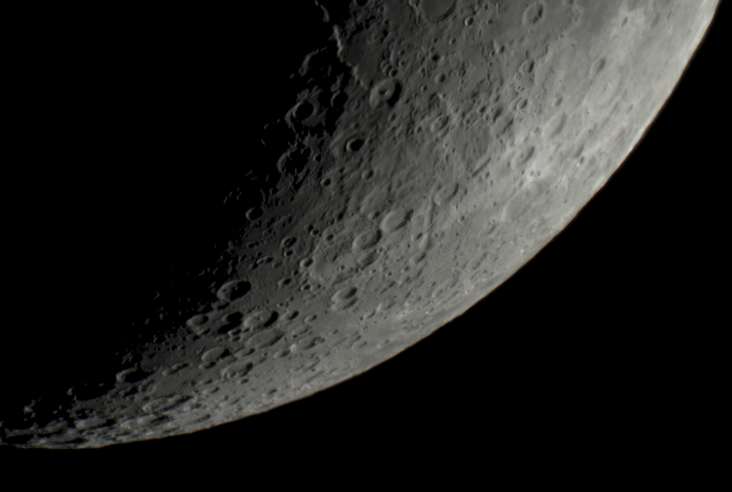
This is important for imaging astronomical objects such as the Sun, Moon and planets with ground-based equipment.

As every observer knows, the ‘seeing’ which depends on atmospheric turbulence, affects how well one can observe the object. Under conditions of very bad seeing, the atmosphere seems to ‘boil’ and the object wobbles about so severely that it is virtually impossible to make a worthwhile observation. However, when seeing conditions are somewhat better; again, as every observer knows, whilst the object still wobbles due to the atmospheric movements, there are rare, fleeting moments of perfect seeing when the observer can see the structure of the object in crystal clarity. Then, the moment is gone, and the observer keeps looking, waiting for the next moment of clarity.

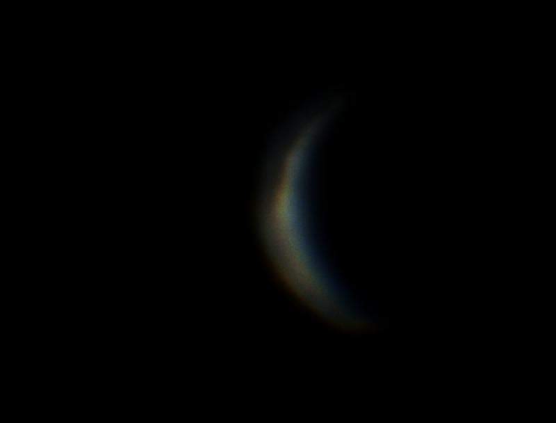
Part of a data set on Venus, played back in slow motion to show the effects of poor seeing


The quality of the seeing, can be ranked on various scales, such as the Antoniadi scale, which was invented by Eugène Antoniadi, a Greek astronomer (1870 to 1944). There are other scales of seeing, but the Antoniadi scale is particularly valuable for planetary observation records.

The Antoniadi Scale of Seeing.
(I.) Perfect seeing, without a quiver.
(II.) Slight quivering of the image with moments of calm lasting several seconds.
(III.) Moderate seeing with larger air tremors that blur the image.
(IV.) Poor seeing, constant troublesome undulations of the image.
(V.) Very bad seeing, hardly stable enough to allow a rough sketch to be made.

Since the advent of electronic imaging devices, it has been possible to image the Sun, Moon and Planets in a totally different way to the imaging that was done using film cameras. Electronic cameras such as CCD cameras and latterly CMOS cameras allow for the rapid acquisition of large numbers of images over a short period of time. With some configurations of camera and telescope, hundreds of frames per second can be captured, each frame effectively freezing the seeing at the moment of time that it was captured.

Turbulence of the air arises from the fact that air packets or cells of different temperature and or humidity refract light to different extents. Shear forces due to winds such as the Jet stream also move the turbulence across the telescope’s line of sight. The above-mentioned variations change the refractive index of the air cells. This changes the apparent positions of tiny regions of the sky (or object) being imaged and causes the image to wobble and shimmer. When light passes from one cell of air to another of differing temperature or humidity, the light is refracted through an angle that causes the apparent movement that is observed as seeing. This is a random process and is described statistically using the Kolmogorov-Tatarski model of turbulence.

Turbulence has several components:

High altitude turbulence associated with the Jet stream.

Geographical turbulence that extends from a few hundred metres to several kilometres. The features of the landscape shape the temperature and humidity of the overlying atmosphere.

Surface turbulence extends from the ground up to several hundred metres and is cause by convection currents arising from a variety of surfaces such as concrete roads, rooftops, vegetation, water etc. This component is responsible for about 50% of the optical distortion.

Instrument turbulence that arises from convection currents inside the telescope itself, the observatory structure and the people in the observatory. Hence the importance of opening the observatory to allow it to cool and allowing the telescope itself to cool down to ambient temperatures before use and never standing underneath the front of the telescope or placing heat generating devices such as computers under the front of the telescope during observing or imaging sessions.

Minimising the effects of Seeing distortions.

This is where the stochastic elements of planetary imaging are used. As mentioned previously; all observers know that by looking carefully at the observed object through the eyepiece, there will be brief moments when the seeing allows the observer to see the detailed structure of the observed object. The better the seeing, the more frequent and the longer duration will these moments of clarity be.

It follows that if one captures high speed images for a long enough period, some of those images will be of much higher quality than others. Indeed, some of the parts of individual images will be of better quality than the rest of the image.

So, the first rule is to capture as many images (or frames in a SER file or an old fashioned AVI file) as you can in a ‘reasonable’ period of time. For some objects, the ‘reasonable’ period of time is quite short. For example, Jupiter, which has a rotation period of 10 hours, rotates so quickly that before very long, rotation will affect the image when the images are combined. Estimates vary, but a reasonable rule is to capture frames of Jupiter for less than 3 minutes.

The captured images (or rather some of them) will be combined or stacked into a single image. This involves accurately registering (i.e placing them exactly one on top of the other) of the images (or even parts of images) before the summing into a stacked image occurs.

Every image has two components; Signal and Noise. Signal is the structure that should be present in every replicate image and noise (which itself has several components) is largely random and thus is different in every image. Noise can be manifest as random small spots in the image due to the electronics of readout and gain etc.

As images are summed into a stack, the signal to noise ratio S/N increases as the noise becomes averaged out over many frames. Increased S/N allows an image to be sharpened to reveal more detail. It can be seen that the S/N as a function of number of stacked images follows the law of diminishing returns.


Thus, for example, whilst there is a 10-fold increase in S/N when one stacks 100 images, there is only a 31.6-fold increase when one stacks 1000 images and a 44.7-fold increase in S/N if one stacks 2000 images. Indeed, stacking 5,000 images only increases the S/N 70.7-fold. So, why capture so many images, if detail can be adequately extracted from fewer (but still a large number) images? In fact, why capture 10,000 or even 20,000 images as we frequently do?

Mathematically, there is no distinction between fine detail and noise. If you try to sharpen an individual frame, this becomes evident as the noise becomes accentuated and the quality of the image decreases. If, however, you try to sharpen a stack of images, the noise has been averaged away and this time, sharpening will accentuate the fine detail which is what is intended. As seen above, the S/N ratio increases as the square root of the number of images stacked.

The answer to the question of why we capture sometimes incredibly large numbers of images lies in the fact that we can rank images according to their quality or sharpness. This ranking can be done automatically by computers and a number of algorithms have been developed to do this. One of the several ways of doing this is to look at a sharp and a blurred image of the same object. In the blurred image, the differences in brightness between adjacent pixels is small, as changes occur gradually across a blurred image. On the other hand, with a sharp image, the differences between adjacent pixels is large, because there are rapid changes in brightness across boundaries within the image. Doing something as simple as summing the difference in brightness of adjacent pixels across the whole image will show a larger sum for the sharp image than it will for the blurred image. This process could be done for all of the images in a data set and the images could be ranked according to their calculated sharpness, from least sharp to most sharp. Then, we could throw away the least sharp images and only stack the sharper images.

AstroDMx Capture for Linux capturing data on the 17.7% crescent Venus on a laptop running Voyager Linux


A relatively good individual frame in the Venus data set

A surface plot of pixel brightness


Horizontally flipped

The lines are very steep, indicating large differences in brightness between adjacent pixels

A relatively poor individual frame in the Venus data set

A surface plot of pixel brightness
Horizontally flipped

Because this is a more blurred image, the lines are less steep, indicating smaller differences between adjacent pixels.

The result of stacking the best 50% of a 5,000-frame SER file without RGB channels alignment
The effects of atmospheric dispersion can be seen in this image, where the Red, Green and Blue components of the image are refracted to different extents.

The results of stacking the same data as those in the previous image but with RGB channels alignment.
This image is unprocessed, other than the RGB channels alignment carried out by Asutostakkert!

Processing of the final stacked image involved wavelet processing in Registax 6 and post processing in the Gimp 2.10.

Final processed image of the 17.6% crescent Venus

Surface plot of the final image
Horizontally flipped

This plot shows the very steep lines, indicating the large adjacent pixel brightness differences of a sharp image

The reason for capturing a huge number of images is that within the data set, there will be a number of good images captured during brief moments of good seeing. The more images we capture, the more good images the data set will contain. We can then afford to throw away many, or even most of the images in the data set and stack just the remaining images of higher quality. We will stack sufficient images to take advantage of the relationship between S/N and number of images stacked. The number of images we throw away is thus as important in a sense, as the number of images we stack.

This is not luck, it was planned, understanding the probabilistic nature of the whole process, by capturing large numbers of replicate images, ranking them on quality and stacking the best. I suppose that if we get a good result after the event, we could be described as having been lucky, and the process could be described as ‘lucky imaging’. However, this is a stochastic process, the outcome of which can vary according to the stochastic processes that have occurred between the light leaving the object to be imaged, passing through the atmosphere with its stochastic turbulence, then the telescope and the final capturing of the images on the sensor. We might be lucky, or we might not, depending on the seeing, but we have been doing Stochastic Imaging!

Thursday 7 May 2020

99.5% waxing Moon and an ISS lunar transit

A Skymax 127 Maksutov was mounted on a Celestron AVX mount. A ZWO ASI178MC fitted with a 0.5 focal reducer was placed at the Cassegrain focus.

Two 5000-frame SER files of two overlapping halves of the 99,5% Moon were captured using AstroDMx Capture for Linux.

The best 50% of frames from each SER file were stacked in Autostakkert!3.1, wavelet processed in Registax 6, stitched into a 2-pane mosaic by Microsoft ICE, and post processed in the Gimp 2.10.

99.5% waxing Moon

Capturing the ISS transit. A Calsky alert informed us that the transit was going to happen and a Stellarium simulation showed the approximate path that the ISS would take across the Moon as seen from our observatory coordinates.

AstroDMx Capture for Linux was used to image the appropriate part of the Moon with enough of the Moon being imaged to allow for any inaccuracies in the predicted path. This is why a focal reducer was used.

Screenshot of AstroDMx Capture for Linux capturing the area of interest.

This screenshot is from the earlier, two-pane capture of the Moon.

In order the capture the transit, the SER file capture was set to manual and was started about a minute before the transit was due to occur.

When the ISS was observed to cross the Moon along a similar, but not identical trajectory predicted by Stellarium, the SER capture was stopped.

SER player was used to process the SER file to optimise the gain and gamma for maximum visibility of the ISS against the lunar background. SER player was then used to isolate the frames containing the ISS and saved them as tiff files. The Tiffs were converted to high quality JPGs and a precise area of the Moon over which the ISS passed was cropped using Nicola's AstroCrop.

The cropped files were then made into an animated Gif using Animation Shop 3.

Animated Gif of the ISS passing in front of the Moon

The ISS passing over Mare Serenitatis

The code refactoring continues, partly as a result of changes made to Ubuntu 20.04, but a new release will be made soon.

Saturday 2 May 2020

M13 with AstroDMx Capture for Linux and Solus Linux

A Skymax 127 Maksutov was mounted on a Celestron AVX GOTO mount. A ZWO178MC 14-bit colour camera, fitted with a 0.5x focal reducer was placed at the Cassegrain focus.

A Thinkpad X230 laptop running Solus was used to capture images of M13 using AstroDMx Capture for Linux.

The equipment

Screenshot of AstroDMx Capture for Linux capturing data on M13

Thirty 30s exposures were captured with matching dark-frames.
The images were stacked in Deep Sky Stacker and post-processed in the Gimp 2.10

M13

Solus is not a Linux distribution that I like, but for running AstroDMx Capture for Linux, it did the job fine.